4Building a Grid Around the Roman Empire’s Northern Border
4.1 Introduction
This notebook constructs a raster grid covering the area around the northern border of the Roman Empire. The goal is to create a spatial dataset that can be used in a regression discontinuity design (RDD): each grid cell gets a distance to the Roman border and an indicator for whether it falls inside or outside the empire.
Working with a regular grid (rather than administrative units like municipalities) is useful because it avoids arbitrary boundaries and allows for a uniform spatial analysis across countries.
We will:
Load the map of Europe and the Roman Empire boundary.
Extract the northern border of the Roman Empire.
Remove a small section of coastline that is not relevant.
Build a 200 km buffer around the northern border.
Clip that buffer to the European land area.
Create a regular grid within this area.
Compute each cell’s distance to the border and its inside/outside status.
Build the signed running variable and visualise the result.
4.2 Step 1: Load packages and spatial data
library(cawd) # historical boundary data (Roman Empire)library(rnaturalearthdata) # country polygonslibrary(tidyverse)
── Attaching core tidyverse packages ──────────────────────── tidyverse 2.0.0 ──
✔ dplyr     1.1.4     ✔ readr     2.1.5
✔ forcats   1.0.0     ✔ stringr   1.6.0
✔ ggplot2   3.5.2     ✔ tibble    3.3.0
✔ lubridate 1.9.4     ✔ tidyr     1.3.1
✔ purrr     1.2.0
── Conflicts ────────────────────────────────────────── tidyverse_conflicts() ──
✖ dplyr::filter() masks stats::filter()
✖ dplyr::lag()    masks stats::lag()
ℹ Use the conflicted package (<http://conflicted.r-lib.org/>) to force all conflicts to become errors
library(sf)
Linking to GEOS 3.10.2, GDAL 3.4.1, PROJ 8.2.1; sf_use_s2() is TRUE
library(nngeo) # nearest-neighbour geometry tools# remotes::install_github("michaeldorman/nngeo") # if not yet installed
We load a map of Europe from Natural Earth and the Roman Empire polygon from cawd.
# Map of Europe (sovereign states)europe <- rnaturalearthdata::sovereignty50 |>st_as_sf() |>filter(continent =="Europe")# Roman Empire at 117 ADre <- cawd::awmc.roman.empire.117.sp |>st_as_sf()
Loading required namespace: sp
4.3 Step 2: Extract the northern border of the Roman Empire
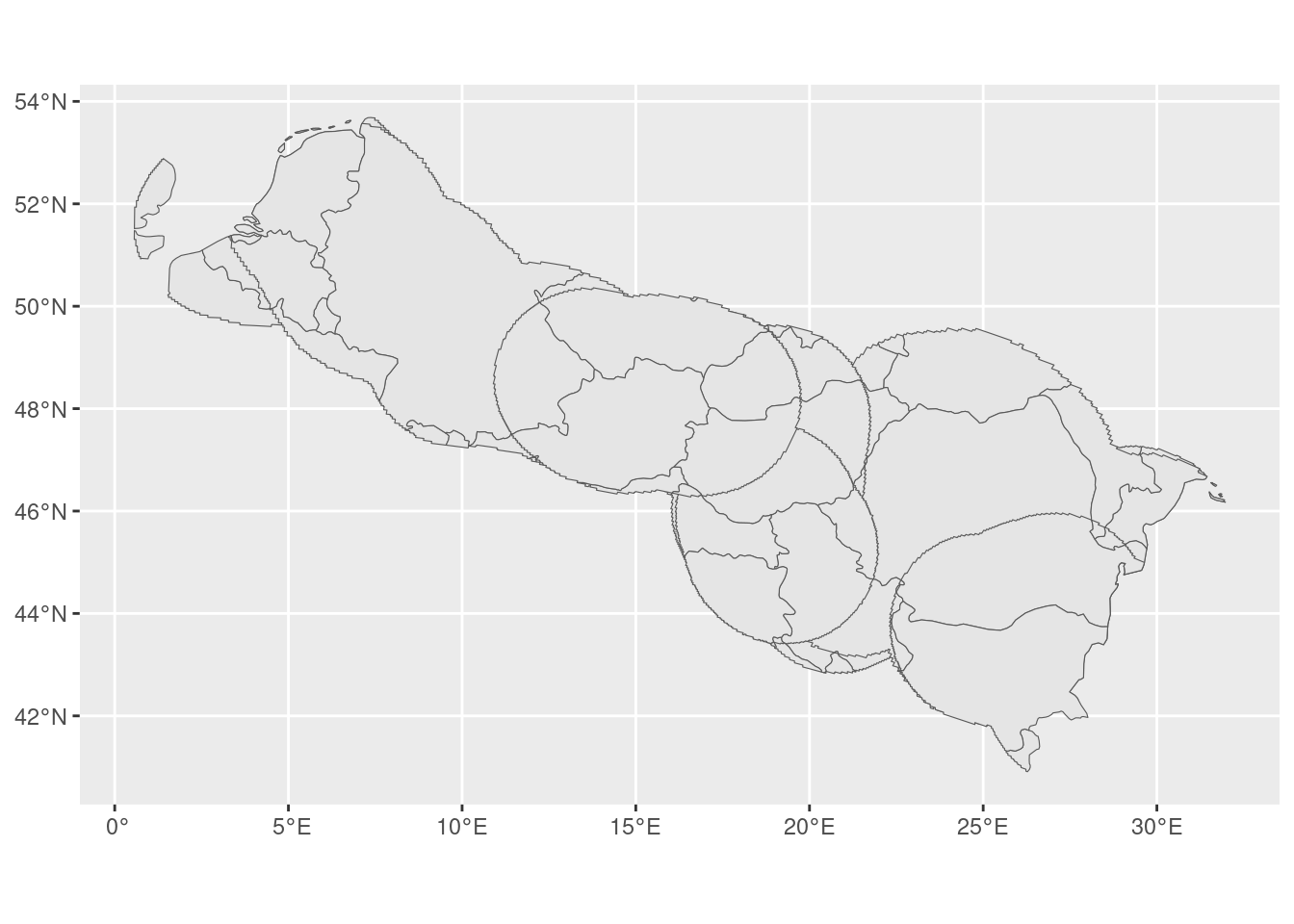
st_boundary() converts the Roman Empire polygon into its outer border (a line). We then clip that line to only the countries that contain the northern frontier — from the Netherlands in the west to Bulgaria in the east.
# Full outer boundary of the Roman Empireboundary_re <-st_boundary(re)# Countries along the northern frontiercountries_with_north_border <- europe |>filter(is.element(sovereignt, c("Netherlands", "Germany", "Croatia","Austria", "Hungary", "Slovakia","Ukraine", "Romania", "Bulgaria","Republic of Serbia" )))# Keep only the border segments that pass through these countriesnorthernmost_lines <-st_intersection(boundary_re, countries_with_north_border)
Warning: attribute variables are assumed to be spatially constant throughout
all geometries
4.4 Step 3: Remove the southern Croatian coastline
The intersection above accidentally picks up part of Croatia’s Adriatic coast, which is a southern border — not the northern frontier we want. We define a small polygon covering that area and subtract it.
Warning: attribute variables are assumed to be spatially constant throughout
all geometries
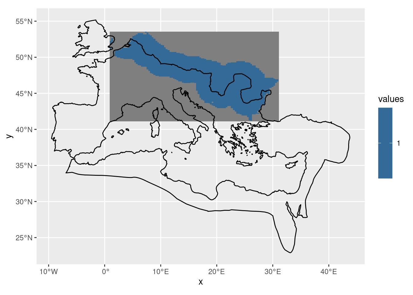
4.5 Step 4: Build a 200 km buffer around the northern border
We want to study areas near the Roman border — within 200 km on either side. st_buffer() creates a band of that width around the border line. We temporarily enable S2 geometry (spherical) for this step, as it is more accurate for wide buffers.
The buffer extends over sea areas that we do not need. We intersect it with the European land polygons to keep only the terrestrial area around the border.
sf_use_s2(FALSE)
Spherical geometry (s2) switched off
area_around_re_border <- europe |>st_intersection(buffer_around_northern_border)
although coordinates are longitude/latitude, st_intersection assumes that they
are planar
Warning: attribute variables are assumed to be spatially constant throughout
all geometries
st_make_grid() lays a 100×100 regular grid over the bounding box of the study area. We then keep only cells that fall within the actual land area (discarding cells over sea or outside our region entirely).
grid <-st_make_grid(area_around_re_border, n =100)# Keep only cells that fall within the study areafilter <-st_within(grid, st_union(area_around_re_border)) |>lengths() >0
although coordinates are longitude/latitude, st_union assumes that they are
planar
although coordinates are longitude/latitude, st_within assumes that they are
planar
final_grid <- grid[filter]
4.8 Step 7: Convert to a raster and save
We convert the grid to a stars raster object (each cell gets a value of 1) and save it as a GeoTIFF for later use.
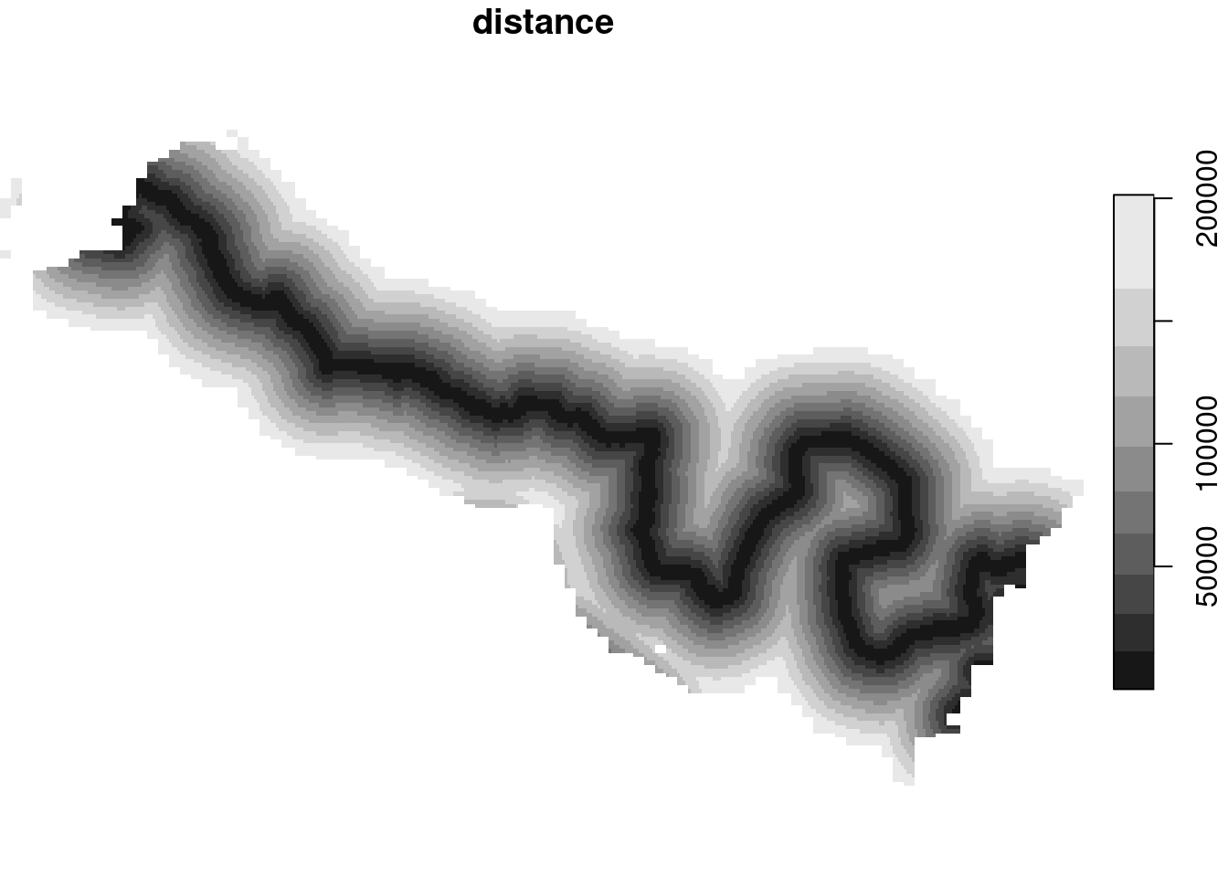
4.9 Step 8: Compute distance to the border for each cell
starsExtra::dist_to_nearest() computes the distance from each raster cell centre to the nearest segment of the northern border line. The result is stored as a new distance attribute on the raster.
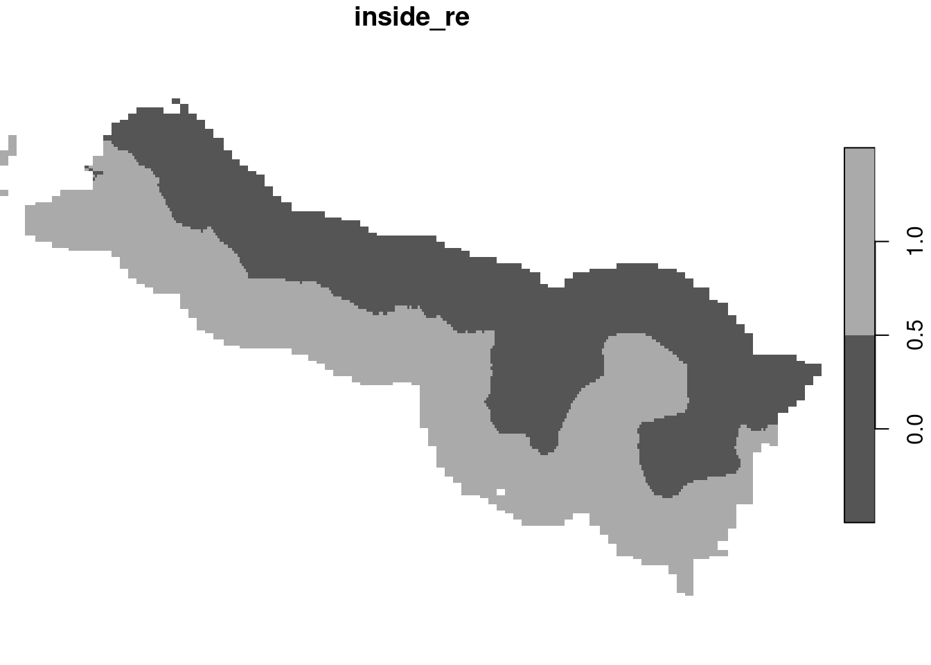
4.10 Step 9: Flag cells as inside or outside the Roman Empire
We convert the raster cell centres to points and use st_within() to check which ones lie inside the Roman Empire polygon. The result is a logical vector that we store as inside_re (1 = inside, 0 = outside, NA = not a valid cell).
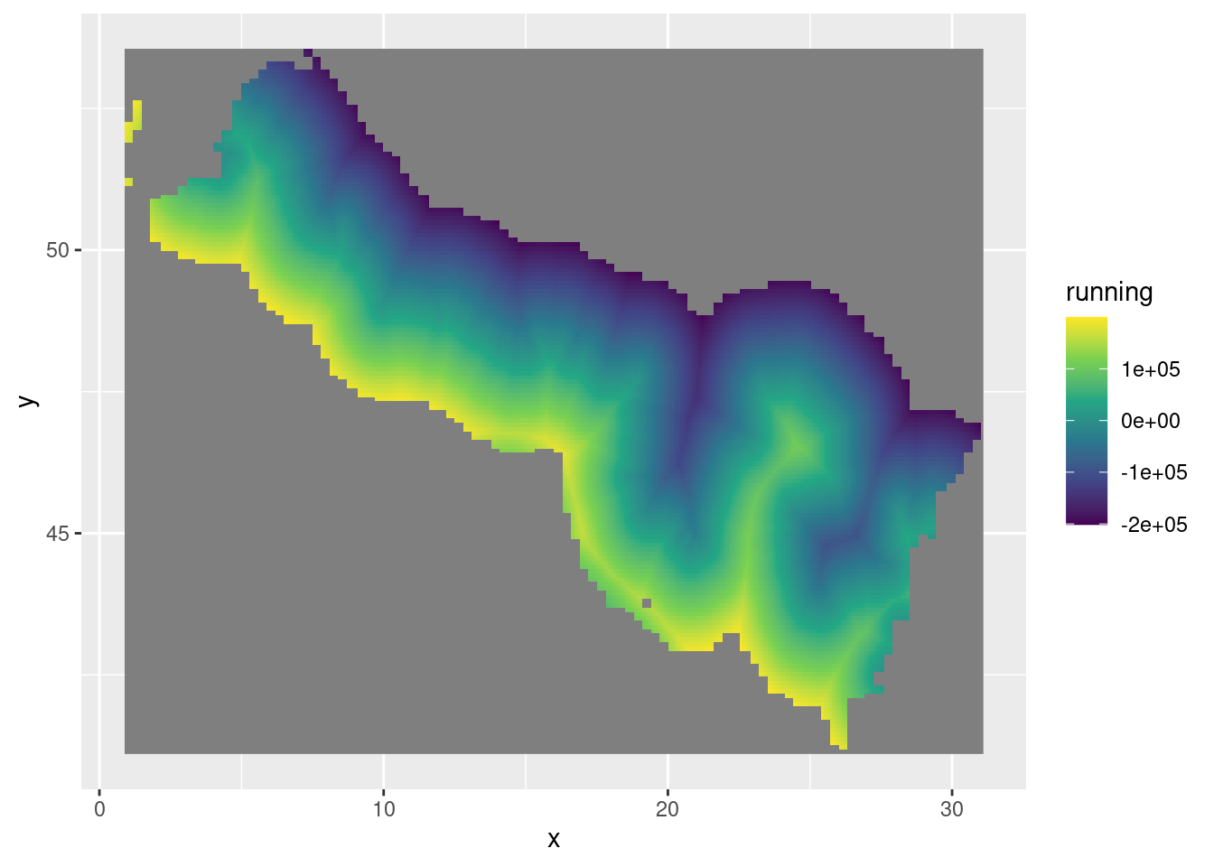
4.11 Step 10: Build the signed running variable and visualise
As in a standard RDD, the running variable is the distance to the border, made positive for cells inside the Roman Empire and negative for those outside.