8Road Infrastructure as a Share of Municipal Area: France
8.1 Introduction
Road density is a common proxy for infrastructure in historical persistence research. A municipality with more roads relative to its area is better connected — and that connectivity may reflect centuries of investment or geographic advantage.
This notebook computes the share of each French municipality’s area covered by roads. The approach is:
Draw a 10-metre buffer around each road segment (approximating its physical footprint).
Intersect those buffers with municipality boundaries.
Sum the buffered road area within each municipality and divide by total municipal area.
The result is a variable between 0 and 1 that can be merged into any France-level dataset for use as a control or outcome.
── Conflicts ────────────────────────────────────────── tidyverse_conflicts() ──
✖ dplyr::filter() masks stats::filter()
✖ dplyr::lag()    masks stats::lag()
ℹ Use the conflicted package (<http://conflicted.r-lib.org/>) to force all conflicts to become errors
library(archive) # for extracting .7z fileslibrary(geodata) # for downloading GADM boundaries
Loading required package: terra
terra 1.8.80

Attaching package: 'terra'

The following object is masked from 'package:tidyr':

    extract
8.3 Step 2: Set up a temporary directory
We download raw data into a temporary directory so nothing is written permanently to the project folder.
tmp <-tempdir()
8.4 Step 3: Download and extract the IGN roads data
The IGN distributes ROUTE500 as a .7z archive. We download it with download.file() and extract it using the archive package, which supports the 7z format.
This file is large (~200 MB) so the download may take a few minutes.
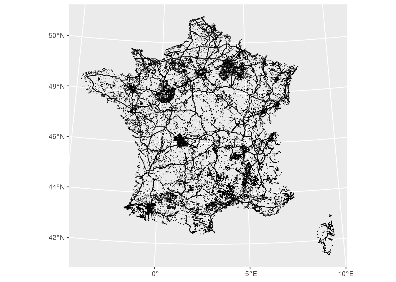
The shapefile we need is TRONCON_ROUTE.shp — each row is one road segment. We filter out segments without a route number (NUM_ROUTE), which removes non-classified tracks. To keep memory use manageable we work with the first 100,000 segments.
# Save the CRS — we will reuse it latercrs <-st_crs(france_routes)
8.6 Step 5: Download municipality boundaries from giscoR
giscoR::gisco_get_lau() downloads LAU (commune-level) boundaries from GISCO. We reproject to match the roads CRS and convert the pre-computed area from km² to m² so it is consistent with st_area() output.
library(giscoR)france_communes <- giscoR::gisco_get_lau(country="France") |>st_transform(crs) |>mutate(total_area = AREA_KM2 *1e6) # convert km² → m² to match st_area() output
8.7 Step 6: Buffer the roads
st_buffer() requires a projected CRS in metres to produce a meaningful buffer distance. We:
Temporarily reproject the roads to UTM zone 30 (metres).
Draw a 10-metre buffer around each segment — approximating its physical road surface.
Reproject the buffers back to the original CRS so they align with the communes.
st_intersection() clips each road buffer to the commune it falls in. The result is a data frame where each row is the piece of a road buffer that lies within a specific commune. We then compute the area of each piece.
We sum the buffered road area within each commune (GISCO_ID is the unique commune identifier in the giscoR LAU dataset), then join the totals back onto the commune data frame.
The road surface share (sufrace) is then capped at 1 (in case rounding or overlapping buffers push it slightly above) and set to 0 for communes with no roads in this subset.
We save the enriched commune dataset as a shapefile. Note that this file only reflects the first 100,000 road segments. To get complete coverage, run the same workflow on the full road network and sum the sufrace columns across all batches.
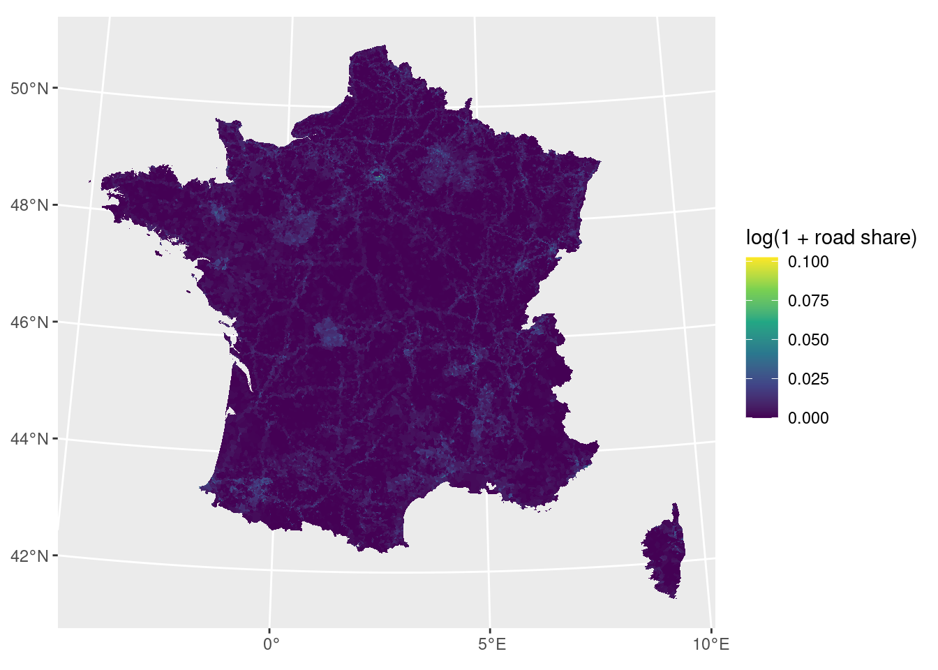
We map the log-transformed road surface share. log(1 + sufrace) compresses the right tail so that the colour scale is not dominated by a few highly urbanised communes.