7  Synthetic Control: The Economic Impact of German Reunification

7.1 Introduction

The synthetic control method is a way to estimate the causal effect of a policy when only a small number of units are treated (e.g. a handful of states or countries). The idea is to build a weighted combination of untreated units — a synthetic version of each treated unit — that closely matches its pre-treatment trajectory. After the treatment, any divergence between the treated unit and its synthetic counterpart is attributed to the policy.

This notebook replicates the classic study of Abadie, Diamond & Hainmueller (2015), which estimates the economic impact of German Reunification (1990) on West Germany’s GDP per capita using the scpi package.

We will:

1. Load and prepare the data.
2. Set up the synthetic control problem with scdata().
3. Estimate the treatment effect with scest().
4. Add uncertainty estimates (confidence intervals) with scpi().

7.2 Step 1: Load packages and data

library(tidyverse)

── Attaching core tidyverse packages ──────────────────────── tidyverse 2.0.0 ──
✔ dplyr     1.1.4     ✔ readr     2.1.5
✔ forcats   1.0.0     ✔ stringr   1.6.0
✔ ggplot2   3.5.2     ✔ tibble    3.3.0
✔ lubridate 1.9.4     ✔ tidyr     1.3.1
✔ purrr     1.2.0     
── Conflicts ────────────────────────────────────────── tidyverse_conflicts() ──
✖ dplyr::filter() masks stats::filter()
✖ dplyr::lag()    masks stats::lag()
ℹ Use the conflicted package (<http://conflicted.r-lib.org/>) to force all conflicts to become errors

library(scpi)

The scpi package ships with the scpi_germany dataset containing annual economic indicators for 17 OECD countries from 1960 to 2003. The treated unit is West Germany, which was reunified with East Germany in 1990.

data("scpi_germany")

7.3 Step 2: Set up the synthetic control problem

scdata() prepares the data structure that scpi needs. The key arguments are:

• id.var, time.var — which columns identify units and time periods.
• outcome.var — the variable we want to predict/compare (gdp).
• period.pre / period.post — pre- and post-treatment time periods.
• unit.tr — the treated unit ("West Germany").
• unit.co — the donor pool of untreated countries.
• features — variables used to match the treated unit to its synthetic in the pre-period.
• cov.adj — additional adjustments applied to the matching (a constant and a linear trend).

donors <- unique(scpi_germany$country)
donors <- donors[donors != "West Germany"]

df <- scdata(
  scpi_germany,
  id.var      = "country",
  outcome.var = "gdp",
  time.var    = "year",
  period.pre  = 1960:1989,
  period.post = 1990:2003,
  unit.tr     = "West Germany",
  unit.co     = donors,
  features    = c("gdp", "infrate", "trade", "schooling", "industry"),
  cov.adj     = list(c("constant", "trend"))
)

7.4 Step 3: Estimate the treatment effect

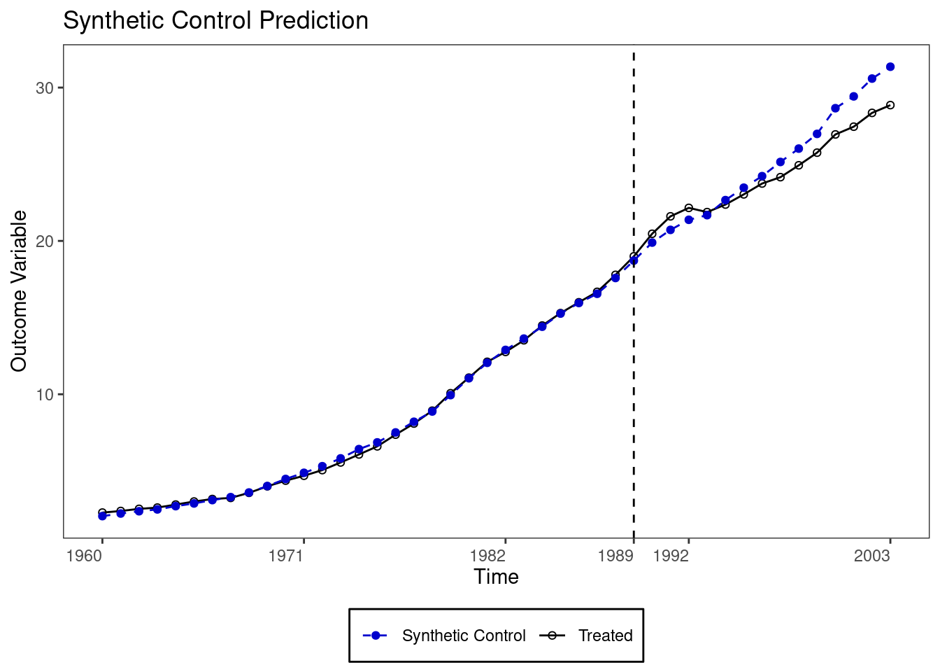
scest() finds the optimal weights for the donor countries. The constraint w.constr = list("name" = "simplex") forces the weights to be non-negative and sum to one — so the synthetic control is a proper convex combination of donors, not an extrapolation.

scplot() then shows the actual outcome alongside the synthetic counterfactual.

res <- scest(df, w.constr = list("name" = "simplex"))
scplot(res)

$plot_out

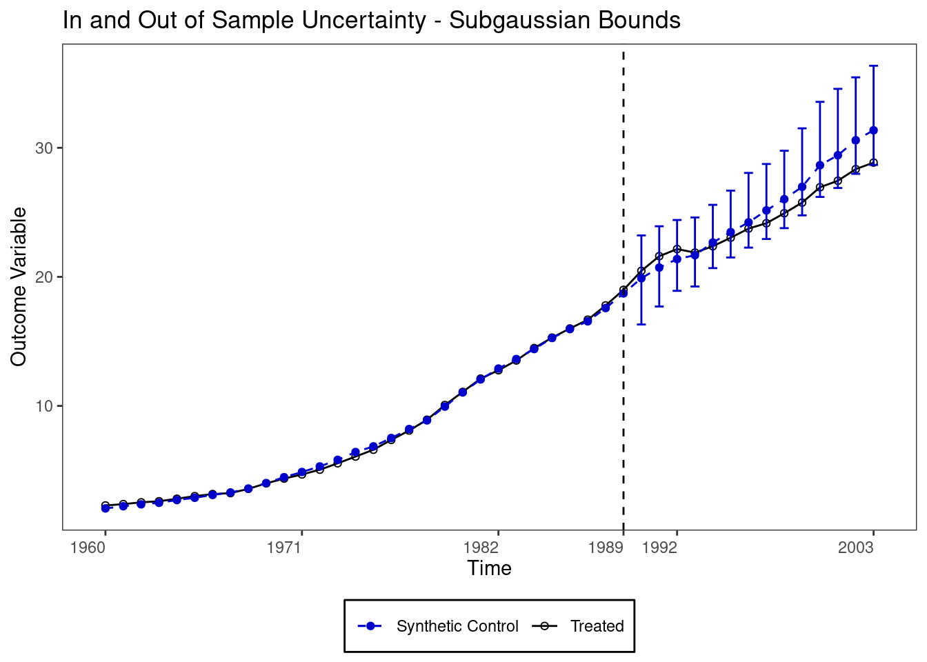
7.5 Step 4: Add uncertainty with bootstrapped confidence intervals

Point estimates alone do not tell us whether the gap between treated and synthetic is statistically meaningful. scpi() adds inference via a Gaussian resampling procedure (e.method = "gaussian"), run in parallel across 4 cores with 50 simulations.

scplot(..., type = "series") shows the time series with confidence bands.

respi <- scpi(df,
              w.constr = list("name" = "simplex"),
              cores    = 4,
              sims     = 50,
              e.method = "gaussian")

---------------------------------------------------------------
Estimating Weights...
Quantifying Uncertainty
Treated unit 1: 5/50 iterations completed (10%) 
Treated unit 1: 10/50 iterations completed (20%) 
Treated unit 1: 15/50 iterations completed (30%) 
Treated unit 1: 20/50 iterations completed (40%) 
Treated unit 1: 25/50 iterations completed (50%) 
Treated unit 1: 30/50 iterations completed (60%) 
Treated unit 1: 35/50 iterations completed (70%) 
Treated unit 1: 40/50 iterations completed (80%) 
Treated unit 1: 45/50 iterations completed (90%) 
Treated unit 1: 50/50 iterations completed (100%) 

scplot(respi)

$plot_out

Note: Increase sims (e.g. to 200 or 1000) for more stable confidence intervals in a real analysis. 50 is used here for speed.